Network Analysis of Exoplanets for NenuFAR SETI
November 4, 2019
Prepared by Caleb Jones and Ross Davis in collaboration with Greg Hellbourg and Ian Morrison for the NenuFAR SETI Project.
The following is a network analysis of 96 exoplanets observed during September 23rd-24th, 2019 by the Search for Extraterrestrial Intelligence (SETI) project that used the French radio telescope NenuFAR.
The network analysis is illustrated through a series of visualizations and tables based on standard statistical techniques used in network analysis. The network analysis can help to narrow the search for technosignatures (signs of ET technology such as radio, optical, or near-infrared signals) by highlighting where a potential technosignature may likely be found in the 96-exoplanet network, according to prominent characteristics of the network as depicted by the visualizations and tables.
The analysis can be used in tandem with other SETI research models to search for exoplanet technosignatures, such as a 3-planet communications model used to identify exoplanet pair-Earth alignments (e.g., heightened focus on alignments that would be within or adjacent to prominent network features).
Network analysis can model information propagation through interconnected systems whether those systems are biological, computer, population, social, or even scientific journals (e.g., Erdős number). Standard statistical techniques associated with network analysis include, yet are not limited to: degree ranking, HITS analysis, and betweenness centrality. In context of SETI, this kind of network analysis can help to narrow the search for technosignatures by examining the composition and distribution of exoplanets as networks.
Additionally, the network analysis can potentially help to enhance non-SETI astronomical research, where networks and the key aspects thereof would be relevant (e.g., quantitatively enhancing interstellar topologies).
Goals
For this initial analysis, the following goals have been identified:
- A 2D visualization with the minimum "max distance" necessary for there to be a single component network (minimum "max distance" is explained in detail in the Network Modeling section herein)
- A visualization with the color of each node based on the effective temperature of the host star
- Visualizing the results of a network community detection
- Comparison of host stars which frequently rank high on various analytical models used to assess a node's importance or influence in a network
- 3D visualization animations of different views from above
Methodology
To achieve these goals the following methodology is used:
- Create network loading logic to read in input data from NenuFAR with nodes as host stars (the input data is
nenufar-seti-field-10-17-19.csvwhich is a customized data file derived from the NASA Exoplanet Archive online). Then experiment with different "max distance" edge values to create a network with a single component - Color host stars in the network using Harvard Spectral Classification from temperature of stars
- Size host stars by number of exoplanets in system
- Visualize the network in 2D dimensionally preserving x/y coordinate positions
- Do a community analysis and colorize host stars based on their respective community ID (modularity class)
- Do Degree, PageRank, HITS, and betweenness centrality analysis to find key star systems in network when modeling information propagation through the network
- Visualize the network with ranked sizing of host stars based on the results of analytical scores
- 3D visualizations of the network preserving x, y, and z dimensions
Network Modeling
To create the network with its nodes and edges, host star systems are loaded from planet data then added to a network. Planets are not modeled as nodes in this network as the distances between planets and their host stars are insignificant compared to interstellar distances. Host stars are effective proxies for their exoplanets when modeling networks at interstellar scale. The number of exoplanets in each system is modeled as an attribute for the host star.
To map positions of host stars onto a Euclidean space (X,Y,Z coordinates) the Astropy library for Python was used to convert from Right Ascension (ra) and Declination (dec) coordinates. The ra/dec coordinates are kept on the host star nodes themselves as attributes, but the distance calculation and visualizations (2D and 3D) use the X/Y/Z Euclidean coordinates.
Straight-line, Euclidean pathways are then calculated between host stars. Rather than include a pathway edge from every host star to every other host star in the network, pathway edges are filtered based on distances which are less than or equal to a "max distance". A max distance is imposed as a way to highlight natural topologies in terms of proximity between host stars. Also, imposing a max edge distance models information relay pathways similar to what emerges in computer networks, biological systems, road systems, or social networks where not every node is connected to every other node but instead utilizes hubs, routers, relays, brokers, and clusters of connections to interact with the wider network. A hypothetical information network between systems may have similar constraints and emergent traits which many other kinds of networks exhibit. An inverse weight is then associated to the edges, giving edges with a smaller distance greater weight which is incorporated into various analysis algorithms.
There is some nuance to determining a minimum max distance to use in the edge modeling. That nuance and the justification for the minimum max distance chosen for this analysis is detailed below in the "Results" section.
Analysis
Once the network is loaded, the following network-wide analysis are done using Gephi. Gephi is an open-source network visualization and analysis platform. For this analysis, the Gephi UI was used (see automation below for ideas on how to automate perhaps using the Gephi Toolkit SDK):
- Degree analysis: both weighted (taking into account edge weights) and unweighted (simple count of edges)
- Community/modularity analysis: to detect subgraphs which are more interconnected than other areas surrounding them - (see: R. Lambiotte, et al, 'Laplacian Dynamics and Multiscale Modular Structure in Networks', 2009)
- HITS analysis: to asses "authority" of a node in the network in terms of information propagation - (see: Jon M. Kleinberg, 'Authoritative Sources in a Hyperlinked Environment', in Journal of the ACM 46 (5): 604–632, 1999)
- Centrality analysis: to rank how often a node appears in pathways in the network - (see: Ulrik Brandes, A Faster Algorithm for Betweenness Centrality, in Journal of Mathematical Sociology 25(2):163-177, 2001)
- PageRank analysis: to score how often random traversals may encounter a node in the network - (see: Sergey Brin, Lawrence Page, The Anatomy of a Large-Scale Hypertextual Web Search Engine, in Proceedings of the seventh International Conference on the World Wide Web (WWW1998):107-117)
Results
Min of Max Distance
After the data was loaded, it became quickly apparent that there are outlier star systems which make a strict "single component" approach untenable. This is illustrated in the histogram in Figure 1, wherein the WTS-1 star system with 1 exoplanet is 3200 parsecs away from our solar system with the next furthest away system being CoRoT-26 which is 1670 parsecs away from our solar system.
Figure 1. Distance from Sun Histogram
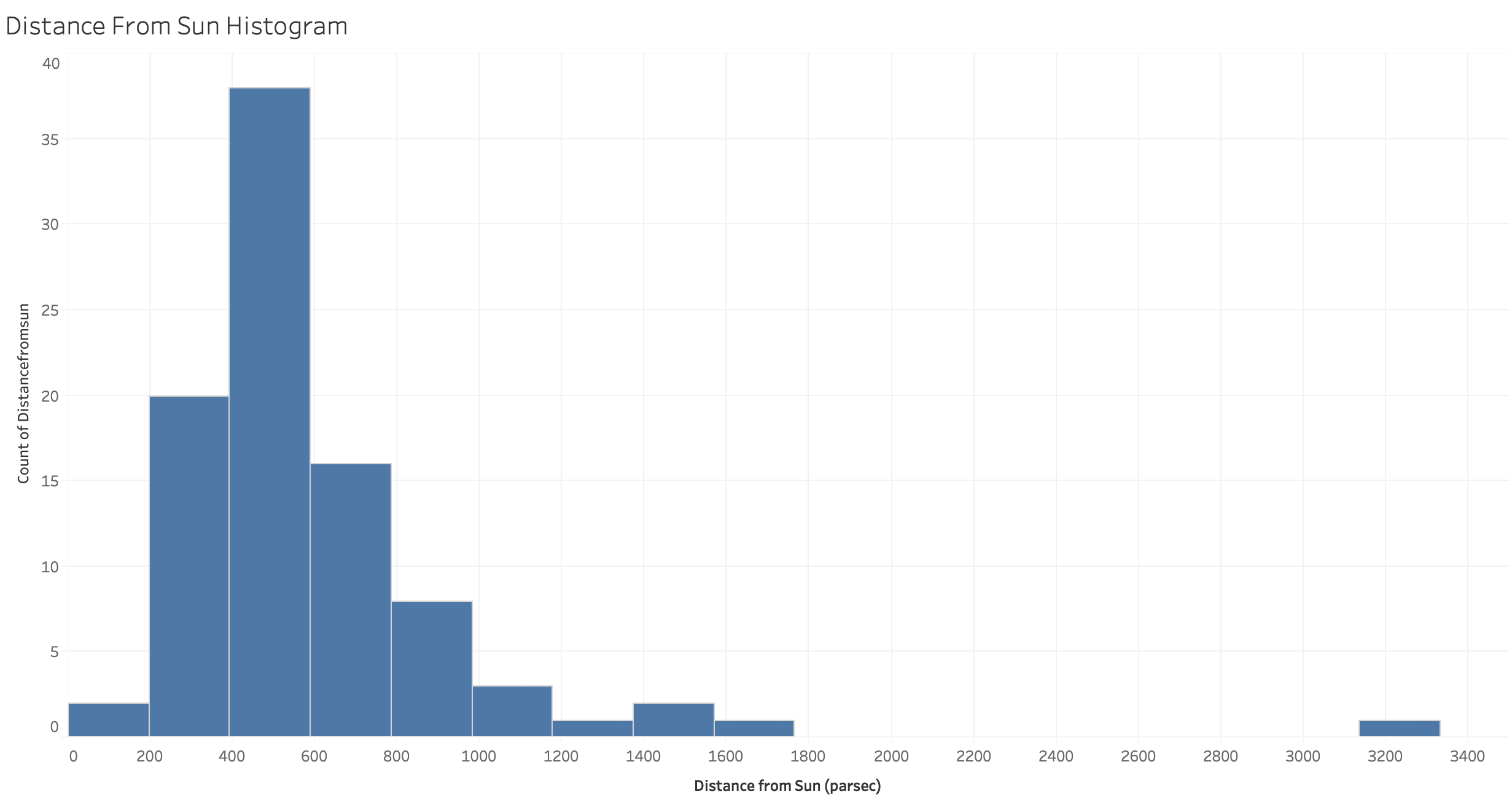
Ideally, a minimum max distance is selected which results in the network having a single connected component, wherein any two nodes are connected via a path. For this dataset, in order to have a network with a single connected component, a minimum edge distance of ~1997 parsecs is required. It is likely this is an artifact of incomplete data as many more exoplanet discoveries and confirmations have yet to be made.
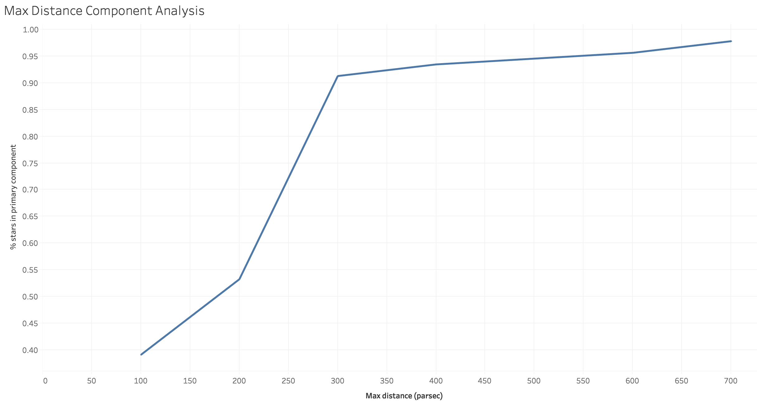
Ignoring WTS-1 and other outliers, a minimum edge distance can be as low as 300 parses while retaining 90% of the host stars in the network. Figure 2 charts the percentage of nodes in the network (y-axis 0.0-1.0) that is included in the largest connected component in the network when different max distance parameters are used (x-axis in parsecs). A "knee" can be seen at around 300 parsecs where diminishing returns are found for higher max edge distances and the primary component drastically shrinks in size much lower than 300 parsecs.
Figure 2. Max Distance Component Analysis
The host stars excluded when using 300 parsecs as an edge max-distance are:
- PSR J1719-1438
- WTS-1
- WTS-2
- CoRoT-26
- V0391 Peg
- BD+20 274
- HD 238914
- WASP-92
For this analysis, a max edge distance of 300 parsecs will be used.
300 Parsecs Network Analysis
Initial Visualization
Figure 3 is a 2D visualization of the resulting 300 parsec network. Host stars are colored as described above (black indicates no temperature data for that star system) and sized based on the number of exoplanets in that system.
Figure 3. 2D network with host stars sized by exoplanet number
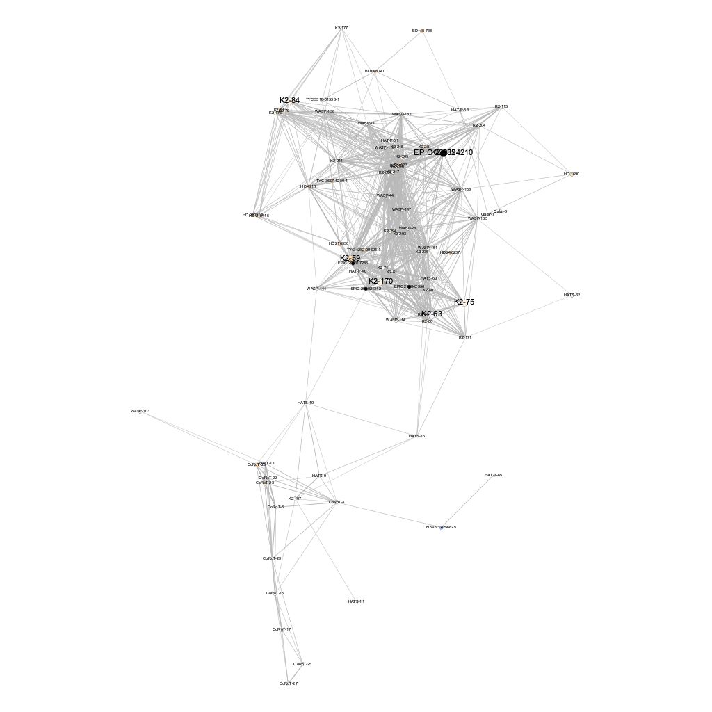
Here, a primary community exists towards the top with a secondary community below.
Modularity/Community Analysis
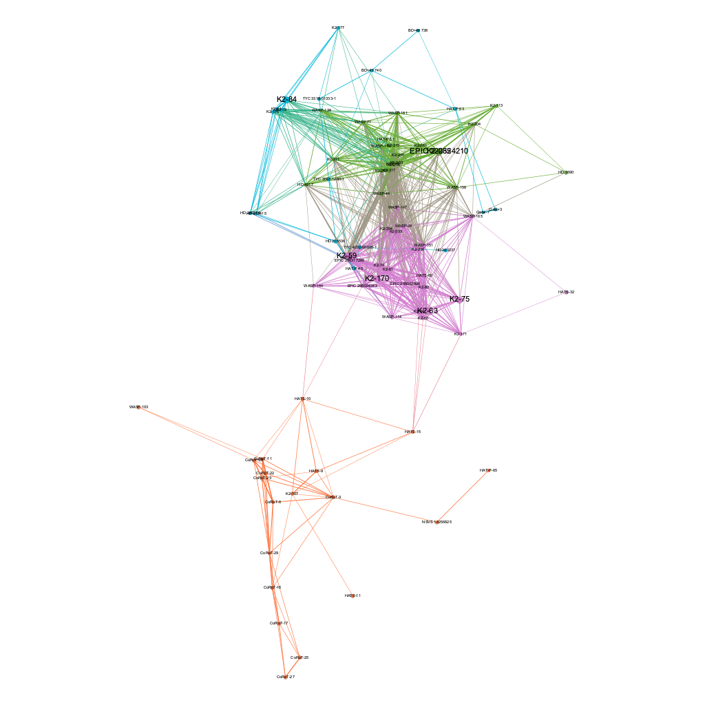
Within this single connected component, a modularity analysis can be done to identify communities of host stars which are more strongly connected to each other compared to the rest of the graph. This analysis takes into account the edge weight calculated above. This results in 4 different communities (using a default resolution parameter of 1.0 for the algorithm). These communities are visualized in Figure 4:
Figure 4. 2D network with host stars and edges colored by community
Degree Analysis
Degree is a measure of the number of edges connected to a given node. The top 10 host stars with the highest degree are ranked in Figure 5:
Figure 5. Top 10 host stars ranked by degree
| Host Star | Degree |
|---|---|
| K2-294 | 42 |
| K2-293 | 41 |
| K2-217 | 41 |
| K2-207 | 41 |
| WASP-44 | 40 |
| WASP-28 | 40 |
| K2-213 | 40 |
| WASP-151 | 40 |
| WASP-147 | 39 |
| WASP-158 | 39 |
An 11th host star also with a degree of 39 is K2-205. A visualization of this ranking is in Figure 6:
Figure 6. 2D network colored by community detection with host stars sized by degree
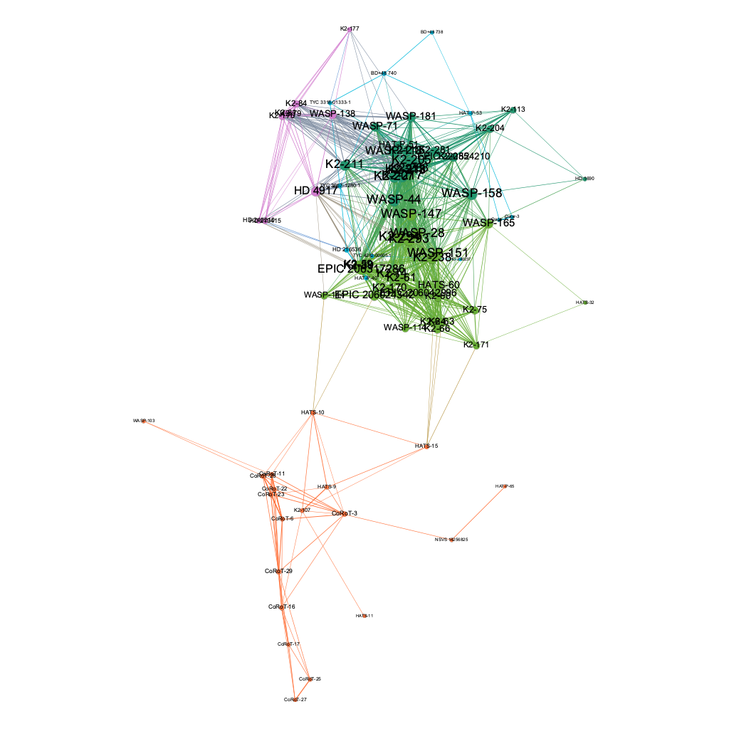
Degree can also be analyzed within the context of communities. Figure 7 shows this ranking:
Figure 7. Top 3 host stars ranked by degree in each community (using color corresponding to community visualization)
- K2-294 (42)
- K2-293 (41)
- WASP-28 (41)
- K2-217 (41)
- K2-207 (40)
- WASP-44 (40)
- HD 4917 (34)
- WASP-138 (25)
- K2-84 (20)
- CoRoT-3 (11)
- CoRoT-29 (10)
- CoRoT-16 (9)
Degree can also be calculated taking into account the weights of edges. Figure 8 ranks the top 10 host stars with the highest weighted degree:
Figure 8. Top 10 host stars ranked by highest weighted degree
- K2-293
- K2-294
- WASP-28
- K2-207
- K2-238
- K2-213
- WASP-44
- K2-217
- K2-74
- K2-218
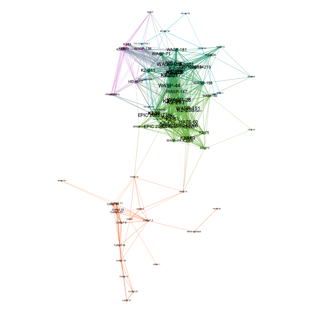
Figure 9 visualizes the network with nodes sized by weighted degree:
Figure 9. 2D network colored by community detection with host stars sized by weighted degree
Holistic Graph Analysis
HITS Analysis
A HITS analysis gives each node two scores: "Authority" and "Hub". "Authority" measures how valuable information stored at that node is and "Hub" measures the value of its edge links. These two scores are defined in terms of one another and thus the algorithm runs repeatedly until a desired convergence is reached. This analysis (using epsilon parameter of 1.0E-4 for the algorithm's convergence limit) results in "authority" scores which closely correlate with the degree of host stars but with some exceptions. Figure 10 shows the top 10 host stars based on their authority score:
Figure 10. Host stars ranked by their HITS authority score - degree included for comparison
| Host Star | Authority | Degree |
|---|---|---|
| K2-294 | 0.190 | 42 |
| K2-293 | 0.187 | 41 |
| WASP-44 | 0.185 | 40 |
| WASP-151 | 0.185 | 40 |
| WASP-28 | 0.184 | 40 |
| WASP-147 | 0.182 | 39 |
| K2-207 | 0.181 | 41 |
| K2-217 | 0.178 | 41 |
| K2-213 | 0.178 | 40 |
| WASP-158 | 0.177 | 39 |
Figure 11 visualizes this ranking:
Figure 11. 2D network colored by community detection with host stars sized by HITS authority score

Centrality Analysis
A Network Diameter analysis gives each node a betweenness centrality score which is a measure of how often that node appears in pathways in the network. This is another metric which can be used to quantify a node's importance or influence in a network (often highlighting broker nodes). Figure 12 shows a ranking of these scores. Figure 13 visualizes these score in the network. Note the prominence of HATS-10 in figure 13 as it brokers connections between two loosely coupled communities in the network. While this prominence might be an artifact of the data (e.g., Are there actually fewer exoplanets in that region of space or have we simply detected fewer?) this methodology is sound in its scoring:
Figure 12. Top 10 host stars ranked by centrality score
- HATS-10
- EPIC 206024342
- HAT-P-51
- CoRoT-3
- K2-107
- HATS-15
- WASP-144
- HAT-P-53
- WASP-114
- CoRoT-11
Figure 13. 2D network colored by community detection with host stars sized by centrality score

PageRank Analysis
Finally, a page rank analysis generates a ranking score based on how likely random traversals are to encounter a node. Like the HITS algorithm, this algorithm is also recursive. An epsilon parameter of 0.001 (for recursion termination) and probability parameter of 0.85 was used for the algorithm. The algorithm is also configured to take into account edge weight. Figure 14 shows this ranking with Figure 15 visualizing the rankings in the network:
Figure 14. Top 10 host stars ranked by PageRank score
- K2-293
- K2-294
- WASP-28
- CoRoT-23
- K2-207
- CoRoT-22
- K2-213
- CoRoT-28
- CoRoT-6
- K2-217
Figure 15. 2D network colored by community detection with host stars sized by PageRank score
![]()
Meta Analysis
Placing the aforementioned types of rankings side by side and comparing how often a host star appears in each can detect whether any particular systems have an importance in the network across these multiple measures (accounting for bias of individual algorithms). This is done in Figure 16. Note that the following table only includes host stars which were in the 2 or more of the top-10 rankings across degree, HITS, or PageRank algorithms. The centrality algorithm's bias produces a non-overlapping top ten for this dataset and so is excluded from this table. Those host stars may deserve special consideration on their own. - indicates that a host star was not in top-10 for that measure:
Figure 16. Ranking of host stars
| Host Star | Degree (rank) | Weighted Degree (rank) | HITS (rank) | PageRank (rank) |
|---|---|---|---|---|
| K2-294 | 1 | 2 | 1 | 2 |
| K2-293 | 2 | 1 | 2 | 1 |
| K2-217 | 3 | 8 | 8 | 10 |
| K2-207 | 4 | 4 | 7 | 5 |
| WASP-44 | 5 | 7 | 3 | - |
| WASP-28 | 6 | 3 | 5 | 3 |
| K2-213 | 7 | 6 | 9 | 7 |
| WASP-151 | 8 | - | 4 | - |
| WASP-147 | 9 | - | 6 | - |
| WASP-158 | 10 | - | 10 | - |
3D Visualization
This network can be visualized in 3D using NAViGaTOR. NAViGaTOR is a network analysis and visualization tool created by the Krembil Research Institute. The latest version (NAViGaTOR 3) does not support 3D visualization of networks. However, the previous version (NAViGaTOR 2.3) does provide that functionality. NAViGaTOR 2.3 (for Windows, Mac, or Linux) can be downloaded here. For this analysis, NAViGaTOR 2.3 only worked on Windows.
When opening a graph file in NAViGaTOR 2.3 (this analysis used GML format), NAViGaTOR 2.3 will, by default, apply a force-directed layout. However, this behavior can be disabled which causes NAViGaTOR 2.3 to use standard graphics properties including any X/Y/Z coordinates. When loading the network (see "Network Modeling" above) the Euclidean X/Y/Z coordinates are stored in this graphics property. Figure 16 shows the results of this 3D visualization.
Figure 16. 3D, rotating visualization of the network using NAViGaTOR 2.3
Data and Artifacts
The following are data and artifacts produced in this project:
Graph/Analysis Data
The following are structured data used or created in this analysis (with the corresponding file format or software used listed in parenthesis):
- Initial input file (CSV)
- Component max-distance data (Libre Office Spreadsheet)
- Network with initial load (Gephi project)
- Network with analysis results (Gephi project)
- Network with analysis results (GML)
- Network analysis results for host stars (CSV)
Visualizations
The following are the 2D network visualizations in scalable vector graphics (SVG) format. This enables arbitrary zooming to see the labels of host stars in the network which are often too small to read in raster image formats like PNG:
- Non community SVG sized by number of planets
- Community SVG
- Degree SVG
- Weighted degree SVG
- HITS SVG
- PageRank SVG
Limitations & Further Development/Application
Much of this data may be biased due to data limitations considering that scientific research involving exoplanets and SETI/technosignatures/astrobiology is still in the formative stages relative to other types of scientific research (i.e., on-going exoplanet discovery and lack of surrounding topology due to missing data for some parameters). While a higher emphasis on systems with exoplanets may give higher weight to systems when modeling hypothetical interstellar networks, systems without planets could serve as relay points. A similar analysis could be done including stars, regardless of exoplanet status, then measure how planetary systems situate relative to key influencing systems. An analysis on a larger body of data which fills out the surrounding space may be able to minimize this bias for this set of stars. One example of such an analysis on a different dataset has been done by Caleb Jones previously. That analysis is published here.
As noted above, default tuning values were used for network-wide analysis algorithms. Additional effort could be made to automatically try several different tuning configurations and comparing results similar to hyperparameter optimization used in tuning neural networks. This process would be different, however, since this process (as is) is not a learning algorithm and could instead create comparison charts looking for plateaus or inflection points in the parameter's effects on the score distributions.
Additional efforts to automate this analysis could be made. In particular, automating the min-of-max edge distance discovery, analysis rankings, and 2D visualizations could almost entirely automate the generation of a report like this. Standardizing the import format or making the loader more dynamic could also accelerate the time necessary to model the network. Besides writing code from scratch to create a 3D file, no practical method for automating the 3D visualization is known and that step may remain a manual process when replicating this anlaysis.
With additional automation, this kind of analysis could be packaged as a general-purpose tool to analyze interstellar structures and/or modeling hypothetical information propagation networks across star systems in the context of SETI research (and potentially non-SETI astronomical research).